Enhancing Categorical Features with Entity Embeddings

Let’s talk about selling beers.

Let’s suppose you are the owner of a pub, and you would like to predict how many beers your establishment is going to sell on a given day based on two variables:

• the day of the week

• the current weather

• We can probably hypothesize that weekends and warm days are going to sell more beers when compared to the beginning of the week and cold days, right? Let’s see if this hypothesis holds to be true

In face of this problem, we usually would start by encoding our categorical data (in this example, the day of the week and the weather) into dummy variables, in order to provide an input to our classifier without any kind of relationship between the existing categorical values.

Our data would look like something below, for the day of week feature (you can imagine something similar for the weather feature):

But does this really makes sense, to treat each categorical value as being completely different from one another, such as when using One-Hot-Encoding? Or even better:

Could we make usage of some sort of technique to “learn” the similarities between each possible value and their outcome?

Entity Embeddings to the rescue

With this given scenario in mind, we can then proceed to the adoption of a technique popularly known in the NLP (Natural Language Processing) field as Entity Embeddings, which allows us to map a given feature set into a new one with a smaller number of dimensions. In our case, it will also allow us to extract meaningful information from our categorical data.

The usage of Entity Embeddings is based on the process of training of a Neural Network with the categorical data, with the ultimate purpose to retrieve the weights of the Embedding layers, allowing us to have a more significant input when compared to a single One-Hot-Encoding approach. By adopting Entity Embeddings we also are able to mitigate two major problems:

• No need to have a domain expert, once we’re capable to train a Neural Network that can efficiently learn patterns and relationships between the values of a same categorical feature, thus removing the step of feature engineering (such as manually giving weights to each day of the week or kind of weather);
• Shrinkage on computing resources, once we’re not longer just directly encoding our possible categorical values with One-Hot-Encoding, which can represent a huge resource usage: Let’s just suppose you have a categorical feature with 10 thousand possible unique values. This would translate into a feature vector with the same amount of empty positions just to represent a given value.

The definition of Entity Embedding

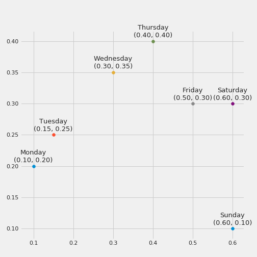
In short words, the Embedding layer is pretty much a Neural Network layer that groups, in a N-dimensional space, categorical values with similar output value. This spatial representation allows us to obtain intrinsic properties of each categorical value, which can be later on used as a replacement to our old dummy encoded variables. If we think about it in a more simple manner, it would mean that days of the week that have a similar output (in our case, number of sold beers), would be close to each other. If you don’t get it, a picture can help:

Here we can see that we have four major groups:

• Group 1, with Monday and Tuesday, possibly related to a low amount of sold beers, due to being the start of the week
• Group 2, with Wednesday and Thursday, with some distance from group 1
• Group 3, with Friday and Saturday, relatively close to group 2, indicating that they show more similarity than when compared with group 1
• Group 4, with Sunday, without many similarities to the other groups

This simple example can show us that the embedding layers can learn information from the real world, such as the most common days for going out and drinking. Pretty cool, isn’t it?

Putting it together with Keras

First of all, we need to know that for using an embedding layer, we must specify the number of dimensions we would like to be used for that given embedding. This, as you can notice, is a hyperparameter, and should be tested and experimented case by case. But as a rule of thumb, you can adopt the number of dimensions as equal to the square root of the number of unique values for the category. So in our case, our representation for the day of the week would have instead of seven different positions, only three (we round up in our case, since the square root of 7 is 2.64). Below we give an example for both mentioned features, as well as add some hidden layers, in order to have more parameters in our model to capture minor data nuances.

# Embedding layer for the 'Day of Week' feature
n_unique_day = df['Day'].nunique()
n_dim_day = int(sqrt(n_unique_day))

input_week = Input(shape=(1, ))
output_week = Embedding(input_dim=n_unique_day, 
                        output_dim=n_dim_day, name="day")(input_week)
output_week = Reshape(target_shape=(n_dim_day, ))(output_week)

# Embedding layer for the 'Weather' feature
n_unique_weather = df['Weather'].nunique()
n_dim_weather = int(sqrt(n_unique_weather))

input_weather = Input(shape=(1, ))
output_weather = Embedding(input_dim=n_unique_weather, 
                           output_dim=n_dim_weather, 
                           name="weather")(input_weather)

output_weather = Reshape(target_shape=(n_dim_weather,))(output_weather)

input_layers = [input_week, input_weather]
output_layers = [output_week, output_weather]

model = Concatenate()(output_layers)

# Add a few hidden layers
model = Dense(200, kernel_initializer="uniform")(model)
model = Activation('relu')(model)

model = Dense(100, kernel_initializer="uniform")(model)
model = Activation('relu')(model)

# And finally our output layer
model = Dense(1)(model)
model = Activation('sigmoid')(model)

# Put it all together and compile the model
model = KerasModel(inputs=input_layers, outputs=model)
model.summary()

opt = SGD(lr=0.05)
model.compile(loss='mse', optimizer=opt, metrics=['mse'])

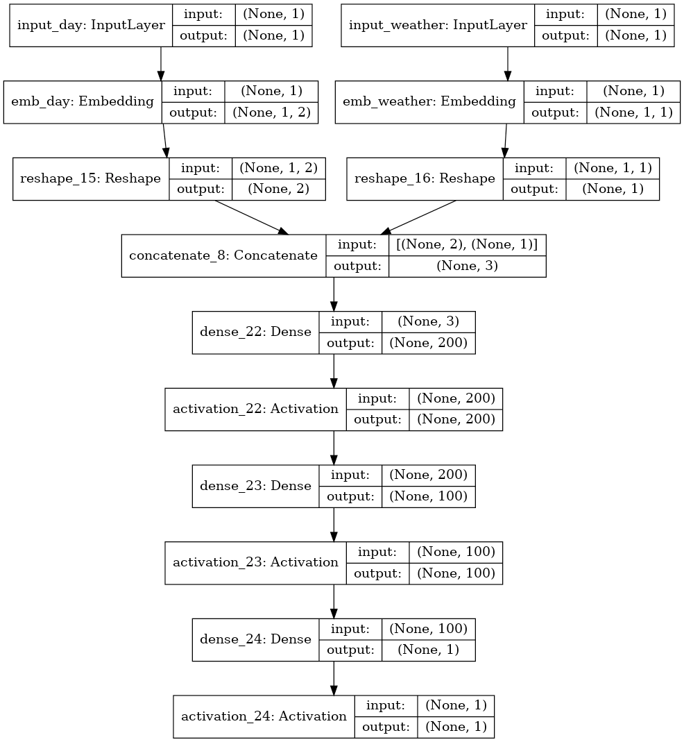
Graphically our Neural Network would have the following representation:

Results

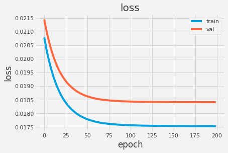
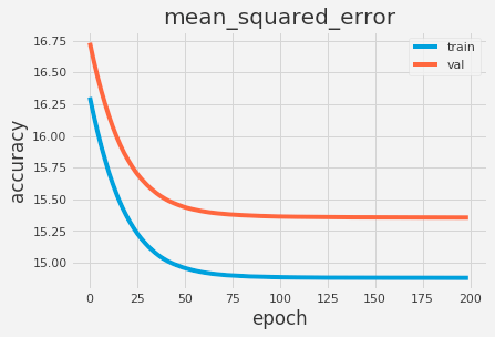
That’s it. We can see that our architecture is composed from a Input layer for each of the categorical values, followed by our Embedding layers, then a Reshape layer and then all put together. Lastly, we add some hidden layers to capture minor nuances of our data. Training our network for 200 epochs with a learning rate of 0.05, we can see some pretty good results for loss and mean squared error:

Conclusions

In this example it may sound silly, but we can again think about our scenario of 10 thousand unique values. The difference between a feature vector with 10 thousand positions (by using One-Hot-Encoding) and another with only 100 (measured by the rule of thumb, when using entity embeddings) is enormous. This is the difference for only a single record for a single feature. You can imagine how complex this becomes with a real world dataset.

If you reached until this point without any doubts, congratulations! But if you do have any kind of questions, suggestions or complains, feel free to reach me

Source Code

If you want to check the full source code for this example, you can find it in my GitHub