Building a multi-output Convolutional Neural Network with Keras
In this post, we will be exploring the Keras functional API in order to build a multi-output Deep Learning model. We will show how to train a single model that is capable of predicting three distinct outputs. By using the UTK Face dataset, which is composed of over 20 thousand pictures of people in uncontrolled environments, we will predict the age, gender and sex for each record presented in the dataset, reaching an accuracy of 91% for gender and 78% for race.
The dataset
The UTKFace dataset is a large dataset composed of over 20 thousand face images with their respectivce annotations of age, gender and ethnicity. The images are properly cropped into the face region, but display some variations in pose, illumination, resolution, etc.
In order to retrieve the annotations of each record, we need to parse the filenames. Each record is stored in the following format: age_gender_race_date&time.jpg
Where:
- age is an integer from 0 to 116
- gender is an integer in which 0 represents male and 1 represents female
- race is an integer from 0 to 4, denoting white, black, asian, indian and others, respectively
- date and time, denoting when the picture was taken
If you want to know more about this dataset, please check their website.
Let’s start by importing some libraries and creating our dictionary to help us on parsing the information from the dataset, along with some other information (dataset location, training split, width and height of the samples).
1
2
3
4
5
6
7
8
9
10
11
12
13
14
15
16
17
18
19
20
21
22
23
24
25
26
27
28
29
import numpy as np
import pandas as pd
import os
import glob
import pandas as pd
import matplotlib.pyplot as plt
import seaborn as sns

dataset_folder_name = 'UTKFace'

TRAIN_TEST_SPLIT = 0.7
IM_WIDTH = IM_HEIGHT = 198

dataset_dict = {
    'race_id': {
        0: 'white',
        1: 'black',
        2: 'asian',
        3: 'indian',
        4: 'others'
    },
    'gender_id': {
        0: 'male',
        1: 'female'
    }
}

dataset_dict['gender_alias'] = dict((g, i) for i, g in dataset_dict['gender_id'].items())
dataset_dict['race_alias'] = dict((r, i) for i, r in dataset_dict['race_id'].items())
Let’s also define a function to help us on extracting the data from our dataset. This function will be used to iterate over each file of the UTK dataset and return a Pandas Dataframe containing all the fields (age, gender and sex) of our records.
1
2
3
4
5
6
7
8
9
10
11
12
13
14
15
16
17
18
19
20
21
22
23
24
25
26
27
28
29
30
31
def parse_dataset(dataset_path, ext='jpg'):
    """
    Used to extract information about our dataset. It does iterate over all images and return a DataFrame with
    the data (age, gender and sex) of all files.
    """
    def parse_info_from_file(path):
        """
        Parse information from a single file
        """
        try:
            filename = os.path.split(path)[1]
            filename = os.path.splitext(filename)[0]
            age, gender, race, _ = filename.split('_')

            return int(age), dataset_dict['gender_id'][int(gender)], dataset_dict['race_id'][int(race)]
        except Exception as ex:
            return None, None, None

    files = glob.glob(os.path.join(dataset_path, "*.%s" % ext))

    records = []
    for file in files:
        info = parse_info_from_file(file)
        records.append(info)

    df = pd.DataFrame(records)
    df['file'] = files
    df.columns = ['age', 'gender', 'race', 'file']
    df = df.dropna()

    return df
1
2
df = parse_dataset(dataset_folder_name)
df.head()
| age | gender | race | file | |
|---|---|---|---|---|
| 0 | 30 | male | asian | UTKFace/30_0_2_20170119183959989.jpg.chip.jpg |
| 1 | 13 | female | others | UTKFace/13_1_4_20170103200733438.jpg.chip.jpg |
| 2 | 36 | male | white | UTKFace/36_0_0_20170104204301875.jpg.chip.jpg |
| 3 | 72 | male | black | UTKFace/72_0_1_20170116205624331.jpg.chip.jpg |
| 4 | 35 | female | white | UTKFace/35_1_0_20170116201535811.jpg.chip.jpg |
| 5 | 80 | female | white | UTKFace/80_1_0_20170110182107291.jpg.chip.jpg |
| 6 | 1 | male | asian | UTKFace/1_0_2_20161219203236876.jpg.chip.jpg |
| 7 | 25 | female | indian | UTKFace/25_1_3_20170119171956657.jpg.chip.jpg |
| 8 | 61 | male | indian | UTKFace/61_0_3_20170109141653583.jpg.chip.jpg |
| 9 | 32 | male | indian | UTKFace/32_0_3_20170119200339548.jpg.chip.jpg |
Data visualization
As an important step to understand not only the distribution of our dataset, but as well the predictions generated by our model, we need to perform some data visualization process on our dataset.
We will start by defining a helper function to generate pie plots based on a given Pandas series:
1
2
3
4
5
6
7
8
9
10
11
import plotly.graph_objects as go

def plot_distribution(pd_series):
    labels = pd_series.value_counts().index.tolist()
    counts = pd_series.value_counts().values.tolist()

    pie_plot = go.Pie(labels=labels, values=counts, hole=.3)
    fig = go.Figure(data=[pie_plot])
    fig.update_layout(title_text='Distribution for %s' % pd_series.name)

    fig.show()
Race distribution
Let’s start by plotting the race distribution with our predefined plot_distribution method.
1
plot_distribution(df['race'])
Having a quick glance at this plot, we can see that almost half of the samples are from the white race, so we can expect this group to have a great accuracy. Other races such as black, indian and asian also show a good number of samples, probably leading us to good accuracy numbers as well. The race ‘others’ (hispanics, latinos, etc) on the other side, show a small number of samples, being more likely to have a small accuracy.
Gender distribution
1
plot_distribution(df['gender'])
For both male and female samples, we have quite a good balanced number of records, so we should have a great accuracy for both classes when using our model.
Age distribution
Let’s also plot how our age feature is distributed over the dataset by using a simple histogram with 20 bins.
1
2
3
4
import plotly.express as px
fig = px.histogram(df, x="age", nbins=20)
fig.update_layout(title_text='Age distribution')
fig.show()
We can also display this same plot in a pie plot. Let’s group the age column into bins and then plot it with a pie chart
1
2
3
4
5
bins = [0, 10, 20, 30, 40, 60, 80, np.inf]
names = ['<10', '10-20', '20-30', '30-40', '40-60', '60-80', '80+']

age_binned = pd.cut(df['age'], bins, labels=names)
plot_distribution(age_binned)
We can observe that our dataset is mostly composed of individuals which age varies between 20 and 30 years, followed by individuals ranging from 30-40 years and then 40-60 years old. These groups represent around 70% of our dataset, so we can believe that we are going to have a good accuracy on predicting individuals in these ranges.
We could also perform some multi-variate analysis on our dataset, but since the scope of this notebook is to demonstrate the usage of a multi-output model with Keras, we won’t be covering it.
Data generator
In order to input our data to our Keras multi-output model, we will create a helper object to work as a data generator for our dataset. This will be done by generating batches of data, which will be used to feed our multi-output model with both the images and their labels. This step is also done instead of just loading all the dataset into the memory at once, which could lead to an out of memory error.
1
2
3
4
5
6
7
8
9
10
11
12
13
14
15
16
17
18
19
20
21
22
23
24
25
26
27
28
29
30
31
32
33
34
35
36
37
38
39
40
41
42
43
44
45
46
47
48
49
50
51
52
53
54
55
56
57
58
59
60
61
62
63
64
65
66
67
68
69
70
from keras.utils import to_categorical
from PIL import Image

class UtkFaceDataGenerator():
    """
    Data generator for the UTKFace dataset. This class should be used when training our Keras multi-output model.
    """
    def __init__(self, df):
        self.df = df

    def generate_split_indexes(self):
        p = np.random.permutation(len(self.df))
        train_up_to = int(len(self.df) * TRAIN_TEST_SPLIT)
        train_idx = p[:train_up_to]
        test_idx = p[train_up_to:]

        train_up_to = int(train_up_to * TRAIN_TEST_SPLIT)
        train_idx, valid_idx = train_idx[:train_up_to], train_idx[train_up_to:]

        # converts alias to id
        self.df['gender_id'] = self.df['gender'].map(lambda gender: dataset_dict['gender_alias'][gender])
        self.df['race_id'] = self.df['race'].map(lambda race: dataset_dict['race_alias'][race])

        self.max_age = self.df['age'].max()

        return train_idx, valid_idx, test_idx

    def preprocess_image(self, img_path):
        """
        Used to perform some minor preprocessing on the image before inputting into the network.
        """
        im = Image.open(img_path)
        im = im.resize((IM_WIDTH, IM_HEIGHT))
        im = np.array(im) / 255.0

        return im

    def generate_images(self, image_idx, is_training, batch_size=16):
        """
        Used to generate a batch with images when training/testing/validating our Keras model.
        """

        # arrays to store our batched data
        images, ages, races, genders = [], [], [], []
        while True:
            for idx in image_idx:
                person = self.df.iloc[idx]

                age = person['age']
                race = person['race_id']
                gender = person['gender_id']
                file = person['file']

                im = self.preprocess_image(file)

                ages.append(age / self.max_age)
                races.append(to_categorical(race, len(dataset_dict['race_id'])))
                genders.append(to_categorical(gender, len(dataset_dict['gender_id'])))
                images.append(im)

                # yielding condition
                if len(images) >= batch_size:
                    yield np.array(images), [np.array(ages), np.array(races), np.array(genders)]
                    images, ages, races, genders = [], [], [], []

            if not is_training:
                break

data_generator = UtkFaceDataGenerator(df)
train_idx, valid_idx, test_idx = data_generator.generate_split_indexes()
Building our model
In this step, we will define our multi-output Keras model. Our model will be composed of three major branches, one for each available feature: age, gender and race.
The default structure for our convolutional layers is based on a Conv2D layer with a ReLU activation, followed by a BatchNormalization layer, a MaxPooling and then finally a Dropout layer. Each of these layers is then followed by the final Dense layer. This step is repeated for each of the outputs we are trying to predict.
These default layers are defined on the make_default_hidden_layers method, which will be reused on building each of the branches of our model. In the code below we will define our class that will be responsible for creating our multi-output model.
1
2
3
4
5
6
7
8
9
10
11
12
13
14
15
16
17
18
19
20
21
22
23
24
25
26
27
28
29
30
31
32
33
34
35
36
37
38
39
40
41
42
43
44
45
46
47
48
49
50
51
52
53
54
55
56
57
58
59
60
61
62
63
64
65
66
67
68
69
70
71
72
73
74
75
76
77
78
79
80
81
82
83
84
85
86
87
88
89
90
91
92
93
94
95
96
97
98
99
100
101
102
103
104
105
106
107
108
109
110
111
112
113
114
115
116
117
118
119
120
from keras.models import Model
from keras.layers.normalization import BatchNormalization
from keras.layers.convolutional import Conv2D
from keras.layers.convolutional import MaxPooling2D
from keras.layers.core import Activation
from keras.layers.core import Dropout
from keras.layers.core import Lambda
from keras.layers.core import Dense
from keras.layers import Flatten
from keras.layers import Input
import tensorflow as tf

class UtkMultiOutputModel():
    """
    Used to generate our multi-output model. This CNN contains three branches, one for age, other for
    sex and another for race. Each branch contains a sequence of Convolutional Layers that is defined
    on the make_default_hidden_layers method.
    """
    def make_default_hidden_layers(self, inputs):
        """
        Used to generate a default set of hidden layers. The structure used in this network is defined as:

        Conv2D -> BatchNormalization -> Pooling -> Dropout
        """
        x = Conv2D(16, (3, 3), padding="same")(inputs)
        x = Activation("relu")(x)
        x = BatchNormalization(axis=-1)(x)
        x = MaxPooling2D(pool_size=(3, 3))(x)
        x = Dropout(0.25)(x)

        x = Conv2D(32, (3, 3), padding="same")(x)
        x = Activation("relu")(x)
        x = BatchNormalization(axis=-1)(x)
        x = MaxPooling2D(pool_size=(2, 2))(x)
        x = Dropout(0.25)(x)

        x = Conv2D(32, (3, 3), padding="same")(x)
        x = Activation("relu")(x)
        x = BatchNormalization(axis=-1)(x)
        x = MaxPooling2D(pool_size=(2, 2))(x)
        x = Dropout(0.25)(x)

        return x

    def build_race_branch(self, inputs, num_races):
        """
        Used to build the race branch of our face recognition network.
        This branch is composed of three Conv -> BN -> Pool -> Dropout blocks,
        followed by the Dense output layer.
        """
        x = self.make_default_hidden_layers(inputs)

        x = Flatten()(x)
        x = Dense(128)(x)
        x = Activation("relu")(x)
        x = BatchNormalization()(x)
        x = Dropout(0.5)(x)
        x = Dense(num_races)(x)
        x = Activation("softmax", name="race_output")(x)

        return x

    def build_gender_branch(self, inputs, num_genders=2):
        """
        Used to build the gender branch of our face recognition network.
        This branch is composed of three Conv -> BN -> Pool -> Dropout blocks,
        followed by the Dense output layer.
        """
        x = Lambda(lambda c: tf.image.rgb_to_grayscale(c))(inputs)

        x = self.make_default_hidden_layers(inputs)

        x = Flatten()(x)
        x = Dense(128)(x)
        x = Activation("relu")(x)
        x = BatchNormalization()(x)
        x = Dropout(0.5)(x)
        x = Dense(num_genders)(x)
        x = Activation("sigmoid", name="gender_output")(x)

        return x

    def build_age_branch(self, inputs):
        """
        Used to build the age branch of our face recognition network.
        This branch is composed of three Conv -> BN -> Pool -> Dropout blocks,
        followed by the Dense output layer.

        """
        x = self.make_default_hidden_layers(inputs)

        x = Flatten()(x)
        x = Dense(128)(x)
        x = Activation("relu")(x)
        x = BatchNormalization()(x)
        x = Dropout(0.5)(x)
        x = Dense(1)(x)
        x = Activation("linear", name="age_output")(x)

        return x

    def assemble_full_model(self, width, height, num_races):
        """
        Used to assemble our multi-output model CNN.
        """
        input_shape = (height, width, 3)

        inputs = Input(shape=input_shape)

        age_branch = self.build_age_branch(inputs)
        race_branch = self.build_race_branch(inputs, num_races)
        gender_branch = self.build_gender_branch(inputs)

        model = Model(inputs=inputs,
                     outputs = [age_branch, race_branch, gender_branch],
                     name="face_net")

        return model

model = UtkMultiOutputModel().assemble_full_model(IM_WIDTH, IM_HEIGHT, num_races=len(dataset_dict['race_alias']))
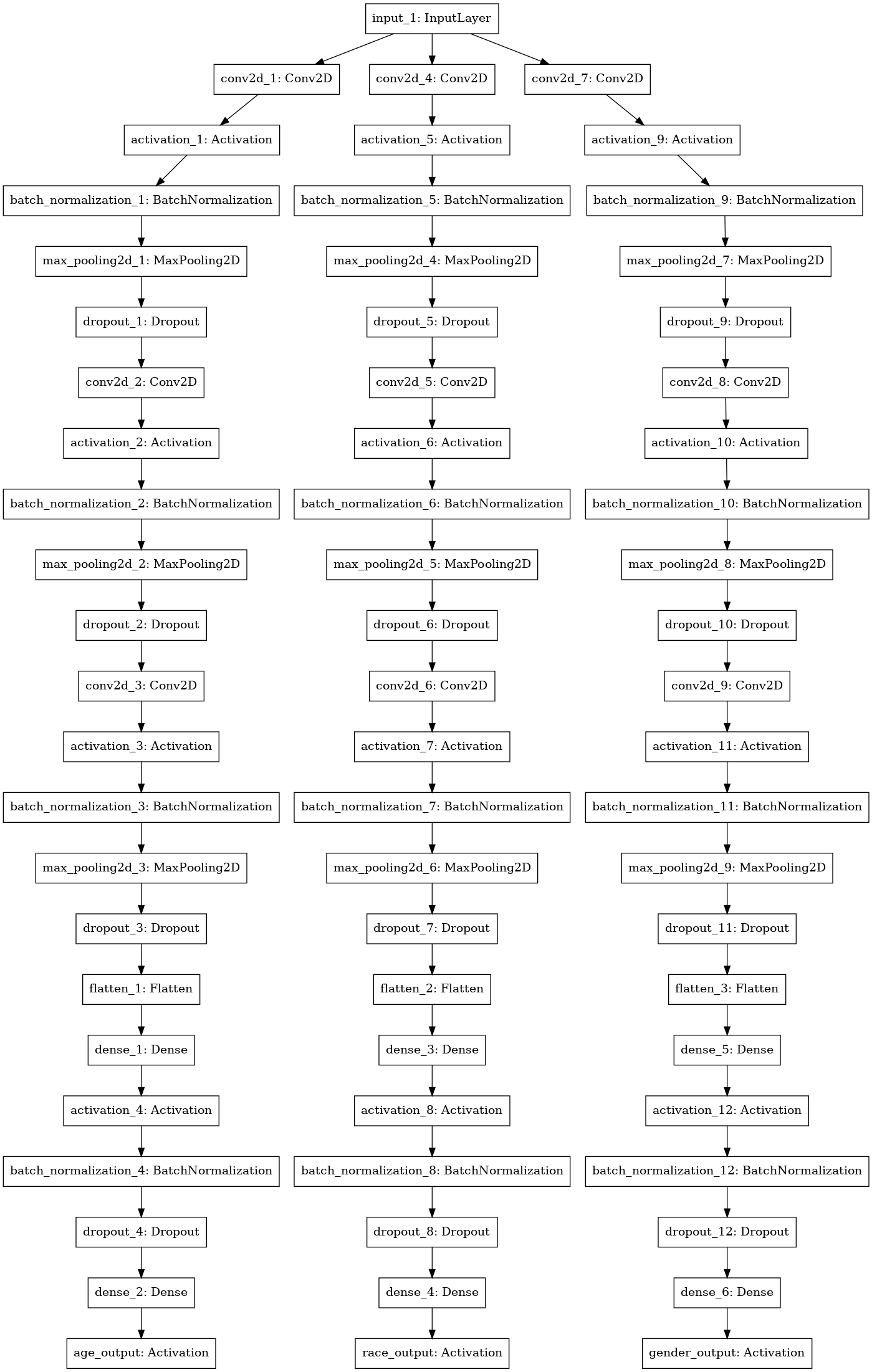
Let’s give a look into our model structure, to have a better understanding of what we are building. We can see from it that we have a single input, that in our case is the image we are feeding the CNN, which does decompose into three separated branches, each with their own Convolutions, followed by their respective Dense layers.
Training our model
Now it’s time to train our multi-output model, once we have both the data ready to use and the model architecture defined. But before doing this step, we need to compile our model. For this task, we will use a learning rate of 0.0004 and an Adam optimizer, but you can be feel free to try with other hyperparameters. We will also use custom loss weights and a custom loss function for each feature.
When building our optimizer, let’s use a decay based on the learning rate divided by the number of epochs, so we will slowly be decreasing our learning rate over the epochs.
1
2
3
4
5
6
7
8
9
10
11
12
13
14
15
16
17
18
19
20
from keras.optimizers import Adam

init_lr = 1e-4
epochs = 100

opt = Adam(lr=init_lr, decay=init_lr / epochs)

model.compile(optimizer=opt,
              loss={
                  'age_output': 'mse',
                  'race_output': 'categorical_crossentropy',
                  'gender_output': 'binary_crossentropy'},
              loss_weights={
                  'age_output': 4.,
                  'race_output': 1.5,
                  'gender_output': 0.1},
              metrics={
                  'age_output': 'mae',
                  'race_output': 'accuracy',
                  'gender_output': 'accuracy'})
Now let’s train our model with a batch size of 32 for both valid and train sets. We will be using a ModelCheckpoint callback in order to save the model on disk at the end of each epoch.
1
2
3
4
5
6
7
8
9
10
11
12
13
14
15
16
17
from keras.callbacks import ModelCheckpoint

batch_size = 32
valid_batch_size = 32
train_gen = data_generator.generate_images(train_idx, is_training=True, batch_size=batch_size)
valid_gen = data_generator.generate_images(valid_idx, is_training=True, batch_size=valid_batch_size)

callbacks = [
    ModelCheckpoint("./model_checkpoint", monitor='val_loss')
]

history = model.fit_generator(train_gen,
                    steps_per_epoch=len(train_idx)//batch_size,
                    epochs=epochs,
                    callbacks=callbacks,
                    validation_data=valid_gen,
                    validation_steps=len(valid_idx)//valid_batch_size)
Once we have our model trained, let’s give a better look into how our model performed on both training and validation sets over the epochs:
Race accuracy
1
2
3
4
5
6
7
8
9
10
11
12
13
14
15
16
17
18
plt.clf()
fig = go.Figure()
fig.add_trace(go.Scatter(
                    y=history.history['race_output_acc'],
                    name='Train'))

fig.add_trace(go.Scatter(
                    y=history.history['val_race_output_acc'],
                    name='Valid'))


fig.update_layout(height=500,
                  width=700,
                  title='Accuracy for race feature',
                  xaxis_title='Epoch',
                  yaxis_title='Accuracy')

fig.show()
We can see that by epoch 50 our model stabilizes itself on the validation set, only increasing on the training one, with an accuracy of approximately 80%.
Gender accuracy
1
2
3
4
5
6
7
8
9
10
11
12
13
14
15
16
17
18
19
20
plt.clf()

fig = go.Figure()
fig.add_trace(go.Scatter(
                    y=history.history['gender_output_acc'],
                    name='Train'))

fig.add_trace(go.Scatter(
                    y=history.history['val_gender_output_acc'],
                    name='Valid'))


fig.update_layout(height=500,
                  width=700,
                  title='Accuracy for gender feature',
                  xaxis_title='Epoch',
                  yaxis_title='Accuracy')


fig.show()
Similarly to the race feature, we can see that our model is able to learn most of the patterns to properly predict the gender from a given individual by the 30th epoch, with an accuracy of approximately 90%.
Age Mean Absolute Error
1
2
3
4
5
6
7
8
9
10
11
12
13
14
15
16
17
18
19
plt.clf()

fig = go.Figure()
fig.add_trace(go.Scattergl(
                    y=history.history['age_output_mean_absolute_error'],
                    name='Train'))

fig.add_trace(go.Scattergl(
                    y=history.history['val_age_output_mean_absolute_error'],
                    name='Valid'))


fig.update_layout(height=500,
                  width=700,
                  title='Mean Absolute Error for age feature',
                  xaxis_title='Epoch',
                  yaxis_title='Mean Absolute Error')

fig.show()
In the task of predicting the age feature, we can see that our model takes around 60 epochs to properly stabilize its learning process, with a mean absolute error of 0.09.
Overall loss
1
2
3
4
5
6
7
8
9
10
11
12
13
14
15
16
17
fig = go.Figure()
fig.add_trace(go.Scattergl(
                    y=history.history['loss'],
                    name='Train'))

fig.add_trace(go.Scattergl(
                    y=history.history['val_loss'],
                    name='Valid'))


fig.update_layout(height=500,
                  width=700,
                  title='Overall loss',
                  xaxis_title='Epoch',
                  yaxis_title='Loss')

fig.show()
We can notice that by the epoch 50 our model starts to stabilize with a loss value of approximately 1.4. There is also a peak in the loss curve which does appear in the Mean Absolute Error for the age feature, which could explain the influence on the learning of the age feature on the overall loss.
Evaluating our model on the test set
In order to assess how our model performs on the test set, let’s use our UTK data generator class, but this time using the test indexes. We will then call the predict_generator method from our trained model, which will output our the predictions for the test set.
1
2
3
4
test_batch_size = 128
test_generator = data_generator.generate_images(test_idx, is_training=False, batch_size=test_batch_size)
age_pred, race_pred, gender_pred = model.predict_generator(test_generator,
                                                           steps=len(test_idx)//test_batch_size)
Let’s iterate one more time over all our test samples, in order to have their labels into a single list. We will also extract the arg max of each record, in order to retrieve the top predictions and ground truths.
1
2
3
4
5
6
7
8
9
10
11
12
13
14
15
16
17
18
19
20
21
test_generator = data_generator.generate_images(test_idx, is_training=False, batch_size=test_batch_size)
samples = 0
images, age_true, race_true, gender_true = [], [], [], []
for test_batch in test_generator:
    image = test_batch[0]
    labels = test_batch[1]

    images.extend(image)
    age_true.extend(labels[0])
    race_true.extend(labels[1])
    gender_true.extend(labels[2])

age_true = np.array(age_true)
race_true = np.array(race_true)
gender_true = np.array(gender_true)

race_true, gender_true = race_true.argmax(axis=-1), gender_true.argmax(axis=-1)
race_pred, gender_pred = race_pred.argmax(axis=-1), gender_pred.argmax(axis=-1)

age_true = age_true * data_generator.max_age
age_pred = age_pred * data_generator.max_age
And finally, let’s print the classification reports for each feature on the test set.
1
2
3
4
from sklearn.metrics import classification_report

cr_race = classification_report(race_true, race_pred, target_names=dataset_dict['race_alias'].keys())
print(cr_race)
1
2
3
4
5
6
7
8
9
10
11
              precision    recall  f1-score   support

       white       0.80      0.91      0.85      2994
       black       0.86      0.82      0.84      1327
       asian       0.86      0.79      0.83      1046
      indian       0.74      0.74      0.74      1171
      others       0.38      0.19      0.25       502

    accuracy                           0.80      7040
   macro avg       0.73      0.69      0.70      7040
weighted avg       0.78      0.80      0.78      7040
From the report above, we can see that our model is really good at predicting asian and black individuals, with a precision of 0.86, followed by white people with 0.80 and indian with 0.74. The race ‘others’ shows a precision of only 0.38, but we need to take into consideration that this group is composed of different races and ethnicities along with a small number of samples, when compared to the other groups. The weighted accuracy for this classification task is 78%, showing that our classifier was able to properly learn patterns to distinguish different types of races.
1
2
cr_gender = classification_report(gender_true, gender_pred, target_names=dataset_dict['gender_alias'].keys())
print(cr_gender)
1
2
3
4
5
6
7
8
              precision    recall  f1-score   support

        male       0.94      0.87      0.91      3735
      female       0.87      0.94      0.90      3305

    accuracy                           0.90      7040
   macro avg       0.90      0.91      0.90      7040
weighted avg       0.91      0.90      0.90      7040
From this report, we can notice that our model is really good at predicting the gender of a given individual, with a weighted accuracy of 91% for this task.
1
2
3
from sklearn.metrics import r2_score

print('R2 score for age: ', r2_score(age_true, age_pred))
R2 score for age: 0.5823979466456328
Example of predictions
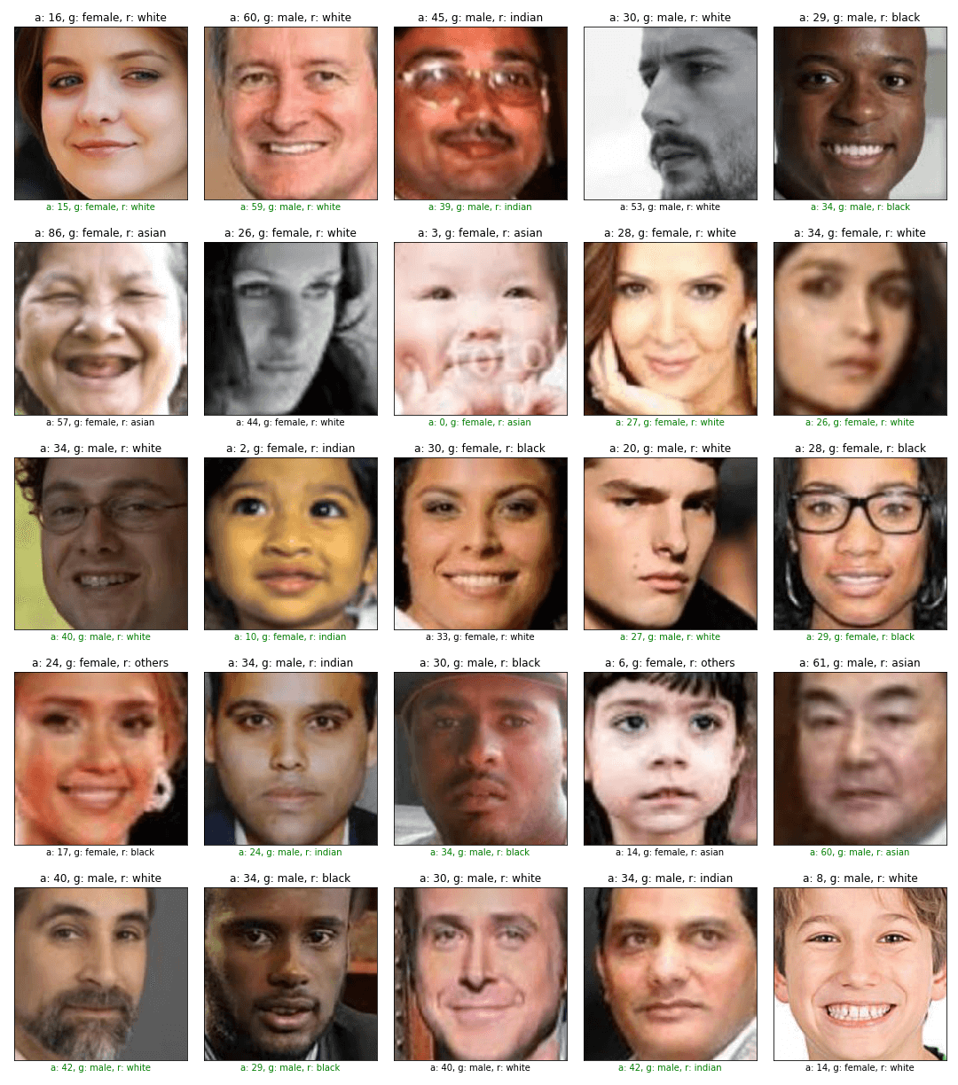
Below we will plot some examples of the performed predictions generated by our model. We can clearly see that our model is really good at predicting gender, race and age, with some minor mistakes for the age feature.
References
UTK Face Dataset: http://aicip.eecs.utk.edu/wiki/UTKFace
Keras Multi-output documentation: https://keras.io/getting-started/functional-api-guide/
SanjayaSubedi post on multi-output model: https://sanjayasubedi.com.np/deeplearning/multioutput-keras/
PyImageSearch post on FashionNet: https://www.pyimagesearch.com/2018/06/04/keras-multiple-outputs-and-multiple-losses/
Plotly: https://plot.ly/


